Some notes on Hessian updating and quasi-Newton methods.
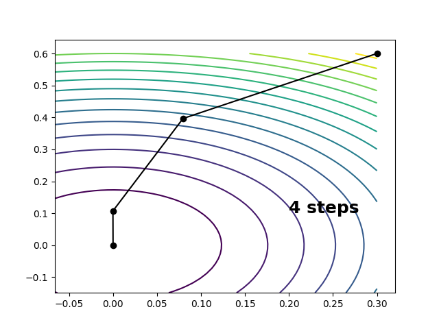
The quadratic approximation of a function \(f\) of several variables \(\mathbf{x}=(x_1, \ldots, x_n)\) at a point looks like this \[ f \approx f_0 + \Delta \mathbf{x}^\mathrm{t} \mathbf{g}_0 + \tfrac{1}{2} \Delta \mathbf{x}^\mathrm{t} \mathbf{H}_0 \Delta \mathbf{x} \] \[ \Delta \mathbf{x} \equiv \mathbf{x} - \mathbf{x}_0 \] where \(f_0\), \(\mathbf{g}_0\), and \(\mathbf{H}_0\) are the function’s value, gradient, and Hessian at \(\mathbf{x}_0\). In this approximation, the Taylor expansion of the gradient is linear \[ \mathbf{g} = \mathbf{g}_0 + \mathbf{H}_0 \Delta \mathbf{x} \] and we can step to the stationary point on our surface by solving for \(\mathbf{g}\overset{!}{=}0\), which gives the following. \[ \Delta\mathbf{x} \overset{!}{=} - \mathbf{H}_0^{-1} \mathbf{g}_0 \] On a perfectly quadratic surface, this will take us to the stationary point in a single step. On a surface with cubic and higher-order components, this step can be repeated iteratively to converge the stationary point to within some threshold of accuracy. This is the Newton-Raphson algorithm for function optimization. An implementation of this alrogithm is shown below. For the following model surface1 \[ f(x, y) = (1 - y^2) x^2 e^{-x^2} + \tfrac{1}{2} y^2 \] the Newton-Raphson algorithm takes us from \( (x, y)=(0.3, 0.6) \) to the minimum at \( (x, y)=(0, 0) \) in four steps:
where the convergence condition is \(\max(\mathrm{abs}(\mathbf{g}))<10^{-5}\).
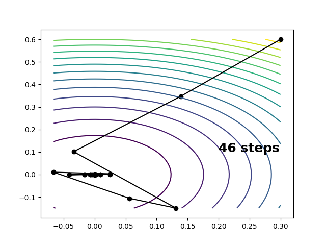
In many cases Hessian matrix evaluations are expensive and the best we can do is calculate gradients at each point. A minimum on the surface can still be reached by gradient descent \[ \Delta\mathbf{x} = - s \frac{\mathbf{g}_0}{|\mathbf{g}_0|} \] where \(s\) determines the step size. Using the step size formula from the wiki for gradient descent gets us to the minimum in 46 steps.
Depending on the relative cost of the derivatives, much of what we save by avoiding the Hessian will be lost by the deterioration in our convergence rate. Furthermore, if the stationary point is a saddle rather than a minimum, gradient following will not get us anywhere.
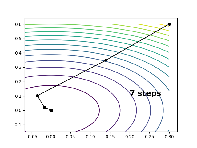
One way around this is to estimate the Hessian on the fly, using only the gradients we calculate along the way. These Hessian estimates can be motivated as follows. The change in the gradient between points \(\mathbf{x}\) and \(\mathbf{x}_0\) sharing a locally quadratic region, satisfies the following. \[ \mathbf{H} \Delta\mathbf{x} \approx \mathbf{H}_0 \Delta\mathbf{x} \approx \Delta\mathbf{g} \] \[ \Delta\mathbf{g} = \mathbf{g} - \mathbf{g}_0 \] This relationship can be used to determine an “update” to the Hessian at \(\mathbf{x}\), starting from an approximation to the Hessian at \(\mathbf{x}_0\), knowing only the gradients. It is known as the secant condition. Denoting the approximate Hessians by tildes, the secant condition is defined as follows. \[ \tilde{\mathbf{H}} \Delta\mathbf{x} \overset{!}{=} \Delta\mathbf{g} \] \[ \tilde{\mathbf{H}} \equiv \tilde{\mathbf{H}}_0 + \Delta\tilde{\mathbf{H}} \] Here we have \(n\) equations and \(n^2\) unknown matrix elements (or rather \(\frac{n(n+1)}{2}\) by symmetry), so the system is underdetermined. The simplest way forward is to parametrize \(\Delta\tilde{\mathbf{H}}\) as a rank-one matrix, which by symmetry must have the form \[ \Delta\tilde{\mathbf{H}} = \eta \mathbf{e} \mathbf{e}^\mathrm{t} \] where \(\eta\) is a scalar and \(\mathbf{e}\) is a unit vector. Substituting this into the secant condition gives \[ \mathbf{e} = \frac{ \Delta\mathbf{g} - \tilde{\mathbf{H}}_0 \Delta\mathbf{x} }{ | \Delta\mathbf{g} - \tilde{\mathbf{H}}_0 \Delta\mathbf{x} | } \] \[ \eta = \frac{ \mathbf{e}\cdot ( \Delta\mathbf{g} - \tilde{\mathbf{H}}_0 \Delta\mathbf{x} ) }{ \mathbf{e}\cdot \Delta\mathbf{x} } = \frac{ ( \Delta\mathbf{g} - \tilde{\mathbf{H}}_0 \Delta\mathbf{x} )^2 }{ ( \Delta\mathbf{g} - \tilde{\mathbf{H}}_0 \Delta\mathbf{x} )\cdot \Delta\mathbf{x} } \] which is known as the symmetric rank-one (SR1) Hessian update. \[ \Delta\tilde{\mathbf{H}}_{\mathrm{SR1}} \equiv \frac{ ( \Delta\mathbf{g} - \tilde{\mathbf{H}}_0 \Delta\mathbf{x} ) ( \Delta\mathbf{g} - \tilde{\mathbf{H}}_0 \Delta\mathbf{x} )^\mathrm{t} }{ ( \Delta\mathbf{g} - \tilde{\mathbf{H}}_0 \Delta\mathbf{x} )\cdot \Delta\mathbf{x} } \] Combining Hessian updating with Newton-Raphson optimization is known as quasi-Newton optimization. By starting from a crude a priori approximation to the Hessian such as2 \[ \tilde{\mathbf{H}}_0 = \frac{|\mathbf{g}_0|}{s} \mathbf{1} \] we can get by with gradients only. For steps within a reasonably quadratic region, \(\tilde{\mathbf{H}}\) will begin to approximate \(\mathbf{H}\) within just a few iterations, substationally improving our rate of convergence relative to gradient descent. For the example above, we make it to the minimum in seven steps.
Codes for everything discussed here can be found on my github, but I’ll paste them here as well for easy reference.
Quasi-Newton algorithm
import numpy
import warnings


def hessian_update_sr1(x, g, x0, g0, h0):
    dx = numpy.subtract(x, x0)
    dg = numpy.subtract(g, g0)
    h0dx = numpy.dot(h0, dx)
    ddg = dg - h0dx

    # avoid division by zero
    if numpy.linalg.norm(dx) < numpy.finfo(float).eps:
        return h0
    else:
        h = h0 + numpy.outer(ddg, ddg) / numpy.dot(ddg, dx)
        return h


def enforce_max_step_size(dx, smax):
    s = numpy.linalg.norm(dx)
    return dx if s < smax else dx * smax / s


def optimize_quasi_newton(x0, func, grad, smax=0.3, gtol=1e-5, maxiter=50):
    dim = numpy.size(x0)

    x0 = numpy.array(x0)
    g0 = grad(x0)
    h0 = numpy.linalg.norm(g0) / smax * numpy.eye(dim)

    converged = False

    traj = [x0]

    for iteration in range(maxiter):
        dx = - numpy.dot(numpy.linalg.pinv(h0), g0)
        dx = enforce_max_step_size(dx, smax)
        x = x0 + dx
        traj.append(x)

        g = grad(x)
        gmax = numpy.amax(numpy.abs(g))
        converged = gmax < gtol

        if converged:
            break
        else:
            h = hessian_update_sr1(x=x, g=g, x0=x0, g0=g0, h0=h0)
            x0 = x
            g0 = g
            h0 = h

    if not converged:
        warnings.warn("Did not converge!")

    return x, traj
Newton-Raphson algorithm
def optimize_newton_raphson(x0, func, grad, hess, smax=0.3, gtol=1e-5,
                            maxiter=50):
    x0 = numpy.array(x0)

    converged = False

    traj = [x0]

    for iteration in range(maxiter):
        g0 = grad(x0)
        h0 = hess(x0)
        dx = - numpy.dot(numpy.linalg.pinv(h0), g0)
        dx = enforce_max_step_size(dx, smax)
        x = x0 + dx
        traj.append(x)

        g = grad(x)
        gmax = numpy.amax(numpy.abs(g))
        converged = gmax < gtol

        if converged:
            break
        else:
            x0 = x

    if not converged:
        warnings.warn("Did not converge!")

    return x, traj
Gradient descent algorithm
def optimize_gradient_descent(x0, func, grad, smax=0.3, gtol=1e-5, maxiter=50):
    x0 = numpy.array(x0)
    g0 = grad(x0)
    s = smax

    converged = False

    traj = [x0]

    for iteration in range(maxiter):
        dx = - s * g0 / numpy.linalg.norm(g0)
        dx = enforce_max_step_size(dx, smax)
        x = x0 + dx
        traj.append(x)

        g = grad(x)
        gmax = numpy.amax(numpy.abs(g))
        converged = gmax < gtol

        if converged:
            break
        else:
            dg = g - g0
            s = numpy.vdot(dx, dg) * numpy.linalg.norm(g0) / numpy.vdot(dg, dg)
            x0 = x
            g0 = g

    if not converged:
        warnings.warn("Did not converge!")

    return x, traj
Model surface
import numpy


def func(z):
    x, y = z
    return (1. - y ** 2) * x ** 2 * numpy.exp(-x ** 2) + 1 / 2. * y ** 2


def grad(z):
    gx = dfdx(z)
    gy = dfdy(z)
    return numpy.array([gx, gy])


def hess(z):
    hxx = d2fdx2(z)
    hxy = d2fdxdy(z)
    hyy = d2fdy2(z)
    return numpy.array([[hxx, hxy], [hxy, hyy]])


def dfdx(z):
    x, y = z
    return 2 * (1. - y ** 2) * x * (1. - x ** 2) * numpy.exp(-x ** 2)


def dfdy(z):
    x, y = z
    return y * (1. - 2 * x ** 2 * numpy.exp(-x ** 2))


def d2fdx2(z):
    x, y = z
    return (2 * (1. - y ** 2) * (1. - 5. * x ** 2 + 2. * x ** 4) *
            numpy.exp(-x ** 2))


def d2fdxdy(z):
    x, y = z
    return -4 * y * x * (1. - x ** 2) * numpy.exp(-x ** 2)


def d2fdy2(z):
    x, y = z
    return 1. - 2 * x ** 2 * numpy.exp(-x ** 2)
Plotting script
import numpy
import matplotlib.pyplot

import algo                         # script with the optimizer functions
from surf import func, grad, hess   # script with the model surface

# Optimize with each algorithm, starting from the following point
x0 = [0.3, 0.6]

x, traj_nr = algo.optimize_newton_raphson(x0=x0, func=func, grad=grad,
                                          hess=hess)

x, traj_qn = algo.optimize_quasi_newton(x0=x0, func=func, grad=grad)

x, traj_gd = algo.optimize_gradient_descent(x0=x0, func=func, grad=grad)

# Generate grid for surface
xmax, ymax = numpy.amax(traj_qn + traj_nr + traj_gd, axis=0)
xmin, ymin = numpy.amin(traj_qn + traj_nr + traj_gd, axis=0)
X = numpy.linspace(xmin, xmax)
Y = numpy.linspace(ymin, ymax)
Z = func(numpy.array(numpy.meshgrid(X, Y)))

# Plot the Newton-Raphson trajectory
matplotlib.pyplot.contour(X, Y, Z, 20)
matplotlib.pyplot.plot(*zip(*traj_nr), color='k')
matplotlib.pyplot.scatter(*zip(*traj_nr), color='k')
s = '{:d} steps'.format(len(traj_nr))
matplotlib.pyplot.text(0.2, 0.1, s=s, fontsize=18, fontweight='bold')
matplotlib.pyplot.savefig('nr')
matplotlib.pyplot.clf()

# Plot the quasi-Newton trajectory
matplotlib.pyplot.contour(X, Y, Z, 20)
matplotlib.pyplot.plot(*zip(*traj_qn), color='k')
matplotlib.pyplot.scatter(*zip(*traj_qn), color='k')
s = '{:d} steps'.format(len(traj_qn))
matplotlib.pyplot.text(0.2, 0.1, s=s, fontsize=18, fontweight='bold')
matplotlib.pyplot.savefig('qn')
matplotlib.pyplot.clf()

# Plot the gradient descent trajectory
matplotlib.pyplot.contour(X, Y, Z, 20)
matplotlib.pyplot.plot(*zip(*traj_gd), color='k')
matplotlib.pyplot.scatter(*zip(*traj_gd), color='k')
s = '{:d} steps'.format(len(traj_gd))
matplotlib.pyplot.text(0.2, 0.1, s=s, fontsize=18, fontweight='bold')
matplotlib.pyplot.savefig('gd')
Footnotes:
-
This generates a gradient-descent of size \(s\) ↩