avcopan.github.io

A brief overview of random variables, building on my previous post about probability theory. Most of this I learned from Wikipedia. As I was writing I got myself terribly confused about the formula for conditional probability densities, so that section is a little wordier and more pedagogical than usual.

Definition 1. A random variable is a well-behaved real-valued function of our sample space, \( X : \Omega \rightarrow \mathbb{R} \).¹

Notation. A common notational convention uses statements containing our random variable as a placeholder to denote events in probability space. These statements are translated according to the following rule. \[ \begin{matrix} \text{‘statement about \(X\)’} \
\updownarrow \
\{\text{all \(\omega\in\Omega\) such that ‘statement about \(X(\omega)\)’ is true}\} \end{matrix} \] Note that this is purely a convenient shorthand. Interpreted as relationships of the function \( X \) these statements are gobbledygook. Another convention we will follow is to use \( f(X) \) to denote the composite random variable \( f\circ X : \Omega \rightarrow \mathbb{R} \), where \( f \) is some function on \( \mathbb{R} \).

Definition 2. The cumulative distribution function (CDF) of \( X \) is defined as \[ \Phi_X(x) \equiv \mathrm{P}(X < x) \] which is a linear combination of step functions when \( X \) is discrete. The event \( X < x \) gradually expands from \( \varnothing \) on the left to \( \Omega \) on the right, so the value of this function increases monotonically from zero to one.

Definition 3. The probability density function (PDF) of \( X \) is the probability per units change in its value. This is the derivative of the CDF \[ \varphi_X(x) \equiv \frac{d}{dx} \Phi_X(x) \] which is a linear combination of Dirac deltas when \( X \) is discrete. By the fundamental theorem of calculus, integrating the PDF from \( x_0 \) to \( x_1 \) gives the probability of the event \( x_0 \leq X < x_1 \), where the equality matters only for discrete distributions. By the unitarity axiom, the integral of the probability density over the whole number line evaluates to one.

Definition 4. The expectation value of a composite random variable \( f(X) \) is \[ \langle f(X) \rangle \equiv \int_\mathbb{R} dx\, \varphi_X(x) f(x) \] where the subscript on the integral denotes the domain of integration. For \( f(X) = X \) this is the mean of \( X \). For \( f(X) = (X - \langle X \rangle)^2 \) this is its variance.

Definition 5. A series of random variables \( X_1, \ldots, X_n \) forms a random vector, \( \mathbf{X} : \Omega \rightarrow \mathbb{R}^n \). The joint cumulative distribution and joint probability density functions of these variables are given by the following \[ \begin{array}{r@{\ }l} \Phi_{\mathbf{X}}(\mathbf{x}) \equiv& \mathrm{P}(\mathbf{X} < \mathbf{x}) \\[10pt] \varphi_{\mathbf{X}}(\mathbf{x}) \equiv& {\displaystyle \frac{ \partial^n \Phi_{\mathbf{X}}(\mathbf{x}) }{ \partial x_1\cdots \partial x_n } } \end{array} \] where the vector inequality denotes an intersection of events, \( \bigcap_i\, X_i < x_i \). Expectation values are determined as usual by integration. \[ \langle f(\mathbf{X}) \rangle \equiv \int_{\mathbb{R}^n} d^n\mathbf{x}\, \varphi_\mathbf{X}(\mathbf{x}) f(\mathbf{x}) \] Note that the function \( f \) need not be scalar-valued. For example, \( f(\mathbf{X}) = (\mathbf{X} - \langle\mathbf{X}\rangle) (\mathbf{X} - \langle\mathbf{X}\rangle)^\dagger \) generates an array of random variables whose expectation value is called the covariance matrix.

When \( f \) only depends on a subset of the variables, \( \mathbf{X}’ \subset \mathbf{X} \), it isn’t immediately obvious that we get the same expectation value from \( \varphi_{\mathbf{X}} \) as we would from \( \varphi_{\mathbf{X}’} \), the marginal density of the relevant variables. Claim 1 below shows that we do. The term “marginal” stems from the fact that the density of the subset can be determined by integrating out the unused variables. For a bivariate distribution displayed on a paper spreadsheet, this was historically done by summing over its rows and columns by hand and writing the totals in the margin of the page.

Definition 6. The conditional cumulative distribution of \( \mathbf{X} \) given \( \mathbf{Y}=\mathbf{y} \) is \[ \Phi_{\mathbf{X}|\mathbf{Y}}(\mathbf{x}|\mathbf{y}) \equiv \mathrm{P}(\mathbf{X}<\mathbf{x}\,|\,\mathbf{Y}=\mathbf{y}) \,. \] The conditional probability density, \( \varphi_{\mathbf{X}|\mathbf{Y}}(\mathbf{x}\,|\,\mathbf{y}) \), is obtained as usual by differentiating this function.² Note that, unless \( \mathbf{Y} \) has a discrete non-zero probability measure at this point, the traditional formula for conditional probabilities is undefined here.

Since the probability of \( \mathbf{Y}=\mathbf{y} \) is necessarily zero for continuous distributions, it may seem strange at first that we can even use this as a conditional statement. In fact, the traditional formula for conditional probabilities is not even defined for \( \Phi_{\mathbf{X}|\mathbf{Y}} \) when \( \mathbf{Y} \) is continuous, because its denominator vanishes. To develop some intuition for how we get around this, think of the plane of this page as a sample space with uniform probability density and consider the events in the following figure.

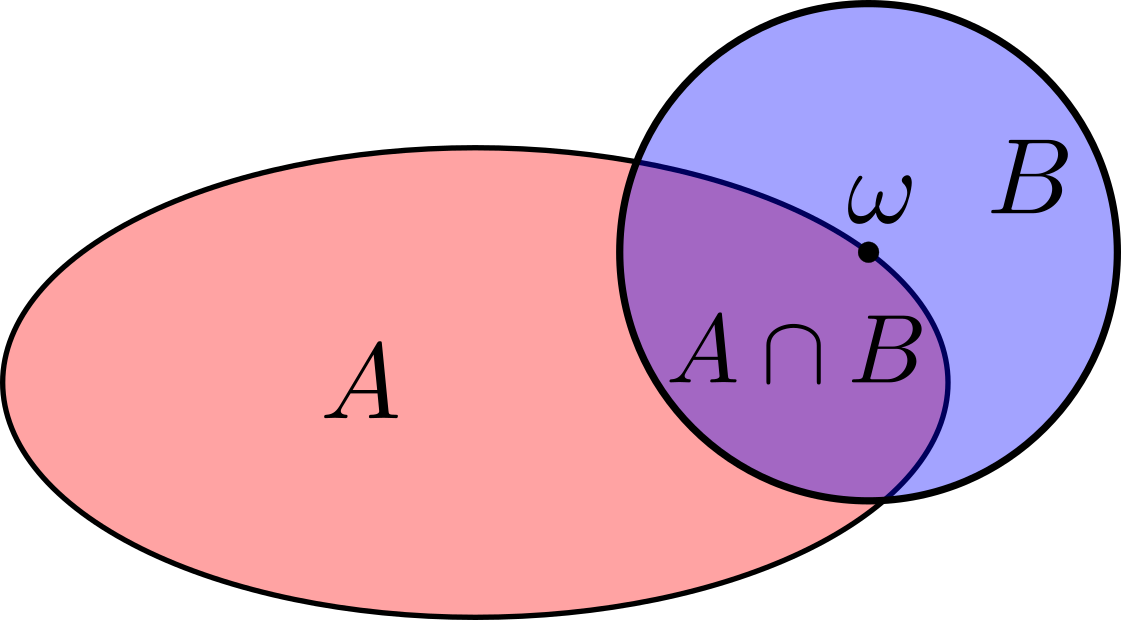
As we shrink the blue disk into the point \( \omega \) at its center, the probabilities of \( B \) and its intersection with \( A \) will approach \( \mathrm{P}(A\,\cap \{\omega\}) = \mathrm{P}(\{\omega\}) = 0 \) as they lose area. But the conditional probability is the ratio of the two, which does not vanish. Instead, it approaches a limiting value of \( \mathrm{P}(A\,|\,\{\omega\}) = \frac{1}{2} \) as the border of the red oval begins to look like a bisecting line at close scale. This qualitative difference in how probabilities vary with respect to arguments versus how they vary with respect to conditions is key in our proof of lemma 1 below.

Definition 7. The random vectors \( \mathbf{X} \) and \( \mathbf{Y} \) are considered independent if the density of one is unaffected by information about the other. This means that, for example, \( \varphi_{\mathbf{X}|\mathbf{Y}}(\mathbf{x}\,|\,\mathbf{y}) = \varphi_{\mathbf{X}}(\mathbf{x}) \) for all \( \mathbf{x} \) and \( \mathbf{y} \). A set of random variables is considered mutually independent if this is true for every pair of non-overlapping subsets.

Claim 1. Margin rule. \({\displaystyle \varphi_{\mathbf{X}}(\mathbf{x}) = \int_{\mathbb{R}^m} d^m\mathbf{y}\, \varphi_{\mathbf{X},\mathbf{Y}}(\mathbf{x}, \mathbf{y}) }\)

Proof: Skipping some post-processing steps,³ we get \[ \int_{\mathbb{R}} dx_1\, \frac{\partial}{\partial x_1} \Phi_{X_1\cdots X_n}(x_1 \cdots x_n) = \Phi_{X_2\cdots X_n}(x_2 \cdots x_n) \] from the fundamental theorem of calculus. Differentiating both sides by \( x_2, \ldots, x_n \) shows that we can delete variables from the PDF by integrating them over their domain. Integrating over the \( \mathbf{Y} \) variables in \( \varphi_{\mathbf{X},\mathbf{Y}} \) completes the proof.

For lemma 1 and the results that follow, assume the random vector \( \mathbf{Y} \) is continuous at \( \mathbf{y} \).

Lemma 1. \(\displaystyle \Phi_{\mathbf{X}|\mathbf{Y}}(\mathbf{x}\,|\,\mathbf{y})\, = \frac{1}{\varphi_{\mathbf{Y}}(\mathbf{y})}\,\, \frac{ \partial^m \Phi_{\mathbf{X},\mathbf{Y}}(\mathbf{x},\mathbf{y}) }{ \partial y_1 \cdots \partial y_m } \)

Proof: Let \( \mathbb{B} \subset \mathbb{R}^m \) be a box centered at \( \mathbf{y} \) with side lengths \( \mathbf{s} \). Then the joint probability of \( \mathbf{X} \) being entrywise less than \( \mathbf{x} \) and of \( \mathbf{Y} \) being in the box is \[ \mathrm{P}(\mathbf{X}<\mathbf{x}\,\cap\,\mathbf{Y}\in\mathbb{B}) = \mathrm{P}(\mathbf{X}<\mathbf{x}\,|\,\mathbf{Y}\in\mathbb{B})\, \mathrm{P}(\mathbf{Y}\in\mathbb{B}) \] by the product rule. As we shrink the sides of the box to teensy microscopic lengths, \( \mathbf{s} \rightarrow d\mathbf{y} \), the marginal and joint probabilities will decrease linearly with the box’s volume, \( d^n\mathbf{y} \). At this zoomed-in scale, the conditional probability becomes independent of the box’s volume and assumes its limiting value at \( \mathbf{Y} = \mathbf{y} \). This reasoning leads to the following equation, which rearranges to the proposed claim after substituting in the relevant distribution and density functions. \[ \frac{ \partial^m \mathrm{P}(\mathbf{X}<\mathbf{x}\,\cap\,\mathbf{Y}<\mathbf{y}) }{ \partial y_1 \cdots \partial y_m }\, d^m\mathbf{y} = \mathrm{P}(\mathbf{X}<\mathbf{x}\,|\,\mathbf{Y}=\mathbf{y})\, \frac{ \partial^m \mathrm{P}(\mathbf{Y}<\mathbf{y}) }{ \partial y_1 \cdots \partial y_m }\, d^m\mathbf{y} \]

Claim 2. \(\displaystyle \varphi_{\mathbf{X}|\mathbf{Y}}(\mathbf{x}\,|\,\mathbf{y}) = \frac{ \varphi_{\mathbf{X},\mathbf{Y}}(\mathbf{x},\mathbf{y}) }{ \varphi_{\mathbf{Y}}(\mathbf{y}) } \)

Proof: Differentiate both sides of lemma 1.

Corollary 1. \(\displaystyle \varphi_{\mathbf{X},\mathbf{Y}}(\mathbf{x},\mathbf{y}) = \varphi_{\mathbf{X}|\mathbf{Y}}(\mathbf{x}\,|\,\mathbf{y})\,\varphi_{\mathbf{Y}}(\mathbf{y}) \)

Proof: Cross-multiply claim 2.

Corollary 2. \(\displaystyle \varphi_{\mathbf{X},\mathbf{Y}}(\mathbf{x},\mathbf{y}) = \varphi_{\mathbf{X}}(\mathbf{x}) \varphi_{\mathbf{Y}}(\mathbf{y}) \) for \( \mathbf{X} \) independent from \( \mathbf{Y} \).

Proof: This follows from corollary 2 and definition 7.

Corollary 3. \(\displaystyle \varphi_{\mathbf{X}}(\mathbf{x}) = \int_{\mathbb{R}^m} d^m\mathbf{y}\,\, \varphi_{\mathbf{X}|\mathbf{Y}}(\mathbf{x}\,|\,\mathbf{y})\, \varphi_{\mathbf{Y}}(\mathbf{y}) \)

Proof: This follows from claim 1 and corollary 1.

Corollary 4. Bayes’ rule III. \(\displaystyle \varphi_{\mathbf{Y}|\mathbf{X}}(\mathbf{y}\,|\,\mathbf{x}) = \frac{ \varphi_{\mathbf{X}|\mathbf{Y}}(\mathbf{x}\,|\,\mathbf{y}) \varphi_{\mathbf{Y}}(\mathbf{y}) }{ \varphi_{\mathbf{X}}(\mathbf{x}) } \)

Proof: This follows from corollary 1 and the symmetry of intersections.

Corollary 4. Bayes’ rule IV. \(\displaystyle \varphi_{\mathbf{Y}|\mathbf{X}}(\mathbf{y}\,|\,\mathbf{x}) = \frac{ \varphi_{\mathbf{X}|\mathbf{Y}}(\mathbf{x}\,|\,\mathbf{y}) \varphi_{\mathbf{Y}}(\mathbf{y}) }{ \int_{\mathbb{R}^m} d^m\mathbf{y}’\,\, \varphi_{\mathbf{X}|\mathbf{Y}}(\mathbf{x}\,|\,\mathbf{y}’) \varphi_{\mathbf{Y}}(\mathbf{y}’) } \)

Proof: This follows from corollaries 3 and 4.

Footnotes: